Cost-Benefit Analysis of Hyperparameter Tuning

Hyperparameter tuning is an effective way to shorten training duration, but tuning itself consumes GPU time and engineering effort, so a cost-benefit assessment is necessary. This document explains a quantitative framework for making this decision.

1. Introduction

When to Tune

Without tuning, you run training with default settings. Defaults are often conservative configurations that prioritize avoiding OOM, and it is not uncommon for them to underutilize hardware performance.

That said, whether to tune is not about finding the technically optimal solution—it is about whether the cost can be recouped through reduced training duration.

In practice, decisions like the following are common:

• Planning a 3-month continued pre-training run—is it worth spending a week on tuning?
• Running SFT weekly—should we invest engineering effort in developing a tuning script?
• Black-box optimization with 100 trials improves the improvement rate, but would 10 heuristic trials be sufficient?

This section organizes these decisions quantitatively, based on training duration, exploration cost, improvement rate, and reuse count.

Scope

The target is tuning that improves training execution time performance. We consider optimizing parallelization strategies (Tensor Parallelism: TP, Pipeline Parallelism: PP, Expert Parallelism: EP, etc.), micro-batch size, recomputation strategies, and similar parameters to improve throughput.

Tuning of hyperparameters that affect model accuracy (learning rate, numerical precision, etc.) is out of scope.

2. Basic Framework for Break-Even Analysis

Whether to tune comes down to comparing "exploration and implementation costs" against "speedup per run × reuse count." The most important variable is the reuse count $R$ (how many times the same optimized configuration is used). The larger $R$ is, the easier it is to recoup your tuning investment.

The Fundamental Inequality

Whether tuning pays off can be determined by the following inequality:

$$\text{Exploration cost} + \text{Implementation cost} < \text{Speedup per run} \times \text{Reuse count}$$

If the right side (speedup) exceeds the left side (cost), tuning is worthwhile. When implementation cost $C = 0$, the decision is based entirely on GPU time, and the following discussion primarily addresses this case.

Variable Definitions

Variable	Meaning	Unit
$X$	Training duration of the job before tuning	Hours (h)
$Y$	Number of GPUs	Count
$Z$	Improvement rate measured after tuning	% (0–100)
$Z_e$	Expected improvement rate estimated before tuning	% (0–100)
$N$	Number of exploration trials	Count
$P$	Execution time per tuning trial (running a short training with a given configuration to measure throughput)	Hours (h)
$R$	Total number of times the optimized configuration is used	Count
$C$	Engineering effort for implementing and validating the tuning script	Person-hours

3. Cost Breakdown

Exploration Cost

$$\text{Exploration cost} = N \times P \times Y \quad [\text{GPU-hours}]$$

For example, running 100 trials of 25 minutes each on 8 GPUs:

$$100 \times \frac{25}{60} \times 8 = 333 \quad \text{GPU-hours}$$

GPU count does not affect the break-even decision

When implementation cost $C = 0$, both the exploration cost and the speedup scale by the same factor $Y$, so GPU count drops out of the break-even equation. However, when implementation cost is included, larger clusters recover that cost faster, so it may not be negligible in operational decisions.

Implementation Cost

$$\text{Implementation cost} = C \quad [\text{person-hours}]$$

$C$ includes:

• Developing the tuning script
• Testing and validation
• Integration into the existing pipeline
• Documentation

Using existing libraries (e.g., ZenithTune's preset feature) keeps effort minimal, while building from scratch requires significant effort. Leveraging libraries is key to reducing $C$. The extension that includes person-hours is covered in Section 5.

Queuing Cost (Qualitative)

Exploration cost is accounted for in GPU-hours, but the indirect cost of cluster occupation during tuning—where other jobs are delayed—is not included in the formula. In environments with high cluster utilization, scheduling tuning runs is also a factor in the decision.

4. Quantifying the Benefits

Speedup per Run

When tuning achieves an improvement rate of $Z$%, the speedup from a single training run is:

$$\text{Speedup per run} = X \times \frac{Z}{100} \quad [\text{hours}]$$

In GPU-hours:

$$\text{Speedup per run (GPU-hours)} = X \times \frac{Z}{100} \times Y$$

For example, if a 720-hour (30-day) training job is improved by 10%, the speedup is 72 hours per run. With $P$ = 25/60 h (25 min) per trial, this is equivalent to $72 / (25/60) \approx 173$ trials worth of exploration cost.

Total Speedup

When the same optimized configuration is used $R$ times, the total speedup is:

$$\text{Total speedup} = R \times X \times \frac{Z}{100} \times Y \quad [\text{GPU-hours}]$$

$R$ is the variable that most affects break-even. Even if $R = 1$ doesn't pay off, $R = 5$ or $R = 20$ may.

Two Key Axes for Algorithm Selection

Changing the tuning algorithm changes both the number of exploration trials $N$ and the improvement rate $Z$. These two variables are the primary axes that determine break-even. The following discussion uses three algorithms as examples:

• Heuristic: An algorithm that narrows down configurations with few exploration trials based on empirical rules. Supported by ZenithTune
• Black-box optimization: An approach that uses Bayesian optimization etc. to automatically search with throughput as the objective function. Supported in ZenithTune via Optuna
• Exhaustive search: Grid search that tries all combinations in the search space

Generally, $N$ increases in this order, and $Z$ tends to increase accordingly, though a good heuristic can achieve high $Z$ with small $N$.

• Initial cost (exploration cost $N \times P$): As $N$ increases, more GPU time is needed for tuning
• Speedup per run ($X \times Z/100$): Higher $Z$ means greater time savings per training run

When choosing an algorithm, verify that the increase in $Z$ from increasing $N$ justifies the increase in exploration cost. The break-even count is:

$$\text{Break-even count} = \frac{\text{Exploration cost}}{\text{Speedup per run}} = \frac{N \times P}{X \times Z / 100}$$

The following chart shows how total speedup accumulates with reuse count $R$ for three algorithms under the conditions $X$ = 150h, $P$ = 25 min. The slope of each solid line represents speedup per run, dotted lines show exploration cost for each algorithm, and circles mark the break-even points.

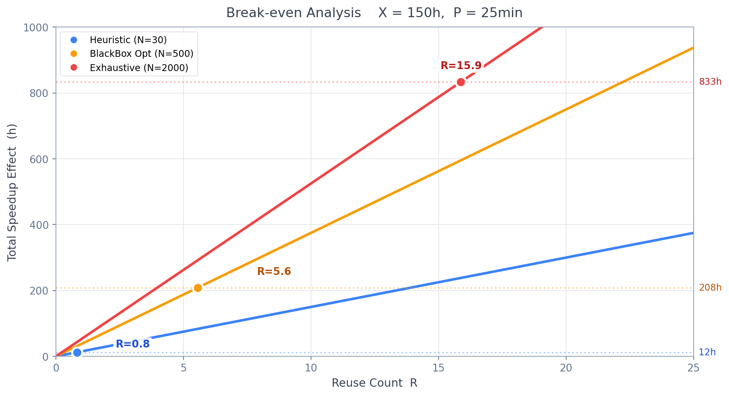
• Heuristic (N=30, Z=10%): Exploration cost ~13h, slope 15.0h/run → break-even at $R \approx 0.8$
• Black-box optimization (N=500, Z=25%): Exploration cost 208h, slope 37.5h/run → break-even at $R \approx 5.6$
• Exhaustive search (N=2000, Z=35%): Exploration cost 833h, slope 52.5h/run → break-even at $R \approx 15.9$

Switching from heuristic to black-box optimization increases the number of exploration trials by ~17x, but the slope (speedup per run) only increases by 2.5x. Whether this additional cost is justified depends on $R$.

Estimating $R$

The value of $R$ varies greatly depending on the nature of the tuning target, so advance estimation is important.

• Small $R$: Pre-training limited to 2–3 runs, one-off fine-tuning of a specific model
• Large $R$: Regularly repeated SFT / reinforcement learning (e.g., grid search over accuracy-related parameters)

To increase $R$, optimize parameters that do not depend on specific models or datasets (e.g., parallelization strategies) and reuse results across the same cluster configuration and framework combination.

5. Derivation Including Implementation Cost

When the cost per GPU-hour is $G$ and the cost per engineer-hour is $W$:

$$N \times P \times Y \times G + C \times W = R \times X \times \frac{Z}{100} \times Y \times G$$

Solving for $R$:

$$R = \underbrace{\frac{N \times P \times 100}{X \times Z}}_{R_{\text{gpu}}} + \underbrace{\frac{C \times W \times 100}{X \times Z \times Y \times G}}_{R_{\text{impl}}}$$

• $R_{\text{gpu}}$: Reuse count needed to recover exploration cost
• $R_{\text{impl}}$: Reuse count needed to recover implementation cost

Because $Y \times G$ appears in the denominator of $R_{\text{impl}}$, larger clusters recover implementation costs faster.

6. Continued Pre-Training vs. Post-Training

Characteristics of the Two Phases

	Continued Pre-Training	Post-Training (SFT / Reinforcement Learning)
Training duration $X$	Large (hundreds to thousands of hours)	Small (hours to tens of hours)
Reuse count $R$	Small (1 to a few)	Large (tens to hundreds)
Cost-effectiveness outlook	Clear (large speedup from a single run)	Unclear (accumulation of small speedups)
Primary decision axis	Is $X \times Z$ large enough?	Is $R$ large enough?

Continued Pre-Training

Continued pre-training spans hundreds to thousands of hours for $X$, so even a small improvement yields a large speedup.

• $X$ = 2160h (90 days), $Z$ = 10% → 216 hours of speedup per run
• Even with an exploration cost of 100 hours ($N \times P$ = 100h), it pays off at $R = 1$

Key considerations:

• $R$ is small (typically 1–3), so the question is "can we recoup in this single run?"
• Since $X$ is large, even a low-cost heuristic can deliver sufficient improvement
• There is room for higher-cost black-box optimization, but since $R$ is small, the cost-effectiveness may not differ much from heuristics

Post-Training (SFT / Reinforcement Learning)

Post-training has small $X$ (hours to tens of hours) but high repetition frequency, so estimating $R$ is the key to the decision.

• $X$ = 10h, $Z$ = 10% → 1 hour of speedup per run
• At $R = 1$, even a 12.5-hour exploration cost (heuristic: $N$ = 30, $P$ = 25 min) cannot be recovered
• However, at $R = 50$, the cumulative speedup of 50 hours makes recovery possible

Even if the speedup per run is small, large $R$ allows cumulative recovery.

Key considerations:

• Estimate how many times you will repeat training with the same configuration
• Low-cost algorithms (heuristics) are particularly advantageous (small exploration cost means fewer runs needed for recovery)
• High-cost algorithms require very large $R$ to be recoverable

Securing Memory Headroom

In post-training, memory consumption can fluctuate due to grid search over accuracy parameters or multi-node execution. Finding a memory-efficient parallelization strategy through tuning can reduce the risk of OOM.

7. Decision Procedure

Step 1: Estimate the Variables

Item	Question
$X$ (Training duration)	How many hours will this job run?
$R$ (Reuse count)	How many times will this optimized configuration be used?
$N \times P$ (Exploration cost)	How much GPU time does the candidate algorithm require?
$Z_e$ (Expected improvement rate)	Based on past results or similar cases, what % improvement is expected?

Step 2: Compute the Break-Even Improvement Rate

From the break-even formula, compute the minimum improvement rate $Z_{\text{break}}$ needed for the investment to pay off:

$$Z_{\text{break}} = \frac{N \times P \times 100}{X \times R}$$

This value represents the threshold: "unless we achieve at least this much improvement, it doesn't pay off."

Step 3: Compare $Z_e$ with $Z_{\text{break}}$ for Each Algorithm

Since $N$ differs by algorithm, $Z_{\text{break}}$ also varies. Compare $Z_e$ and $Z_{\text{break}}$ for each algorithm, then choose from those that are profitable based on cost-effectiveness.

Z_e significantly exceeds Z_break → Proceed with tuning using that algorithm
Z_e is roughly equal to Z_break  → Consider switching to a lower-cost algorithm
Z_e is below Z_break             → That algorithm does not pay off

When unsure about algorithm choice

When in doubt, start with the lowest-cost algorithm (heuristic or black-box optimization with limited exploration trials). This is the safest approach.

• Low exploration cost means low downside risk
• The measured improvement rate $Z$ can inform decisions about investing in higher-cost algorithms

When unsure about estimating improvement rate and reuse count

Estimating $Z_e$ requires GPU profiling expertise. By leveraging AIBooster's Performance Observability (PO), you can visualize GPU utilization, SM core utilization, and other metrics, enabling a rough estimate of $Z_e$ even without dedicated profiling. Estimating $R$ requires visibility into the overall project plan. Consulting with specialists experienced in GPU workload optimization is also an option.

8. Summary

Estimate the four variables in the fundamental inequality—$X$, $R$, $N \times P$, $Z_e$—and make your decision. The question is not "to tune or not to tune" but "which algorithm, at what cost." ZenithTune provides multiple algorithms with varying cost and speedup characteristics to help answer this question. Choose the algorithm that best balances cost and speedup for your use case.