Improving Performance

This guide explains how to observe and analyze various metrics on AIBooster and how to improve performance, using a case study of continued pre-training of Llama4 Scout.

Environment and Configuration

Training Environment

• Koukaryoku PHY Sec.A x 4 nodes
  • GPU: NVIDIA H100 80GB x 8
  • Interconnect: 200Gbps x 4
  • Ubuntu 22.04 LTS
• Initial setup completed with AIBooster
  • Performance observation dashboard/profiling tools
  • Performance improvement framework
  • Recommended infrastructure settings applied
  • Model development kit

Training Configuration and Prerequisites

• Training library: LLaMA-Factory
• Dataset: RedPajama-V1 ArXiv Subset (28B Token Count)
• Using configuration values from the official sample (Llama3 full parameter SFT), changing only the model
• After deploying code, model, and data, execute the following command on each node

FORCE_TORCHRUN=1 \
  NNODES=4 \
  NODE_RANK=<node number 0..3> \
  MASTER_ADDR=<address of node 0> \
  MASTER_PORT=29500 \
  llamafactory-cli train examples/train_full/llama4_full_pt.yaml

• Training completed in approximately 28 hours for 3 epochs

Training completed. Do not forget to share your model on huggingface.co/models =)


{'train_runtime': 100892.0068, 'train_samples_per_second': 1.199, 'train_steps_per_second': 0.019, 'train_loss': 1.72523823162866, 'epoch': 3.0}
100%|███████████████████████████████████████████████████████████████████████████████████████████████████████████████████████████████████████████████████| 1890/1890 [28:01:32<00:00, 53.38s/it]
[INFO|trainer.py:3984] 2025-04-28 08:27:36,306 >> Saving model checkpoint to saves/llama4-109b/full/pt

..snip..

[INFO|tokenization_utils_base.py:2519] 2025-04-28 08:32:00,528 >> Special tokens file saved in saves/llama4-109b/full/pt/special_tokens_map.json
***** train metrics *****
  epoch                    =             2.996
  total_flos               =         1557481GF
  train_loss               =            1.7252
  train_runtime            = 1 day, 4:01:32.00
  train_samples_per_second =             1.199
  train_steps_per_second   =             0.019
Figure saved at: saves/llama4-109b/full/pt/training_loss.png
[WARNING|2025-04-28 08:32:00] llamafactory.extras.ploting:148 >> No metric eval_loss to plot.
[INFO|modelcard.py:450] 2025-04-28 08:32:00,937 >> Dropping the following result as it does not have all the necessary fields:
{'task': {'name': 'Causal Language Modeling', 'type': 'text-generation'}}

Analysis of Collected Metrics

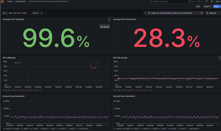
Results from observing time-series metrics on the AIBooster performance observation dashboard:

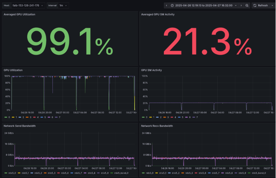
• Average GPU Utilization: 99.1% (appears high at first glance)
• Average GPU SM Activity: 21.3% (GPU core utilization efficiency is low in the 20% range and flat)
• GPU Utilization, GPU SM Activity: GPU stalls at regular intervals
• Network Send/Recv Bandwidth: Interconnect bandwidth usage averages around 6GB/s for both Send/Recv (theoretical bandwidth is 25GB/s)

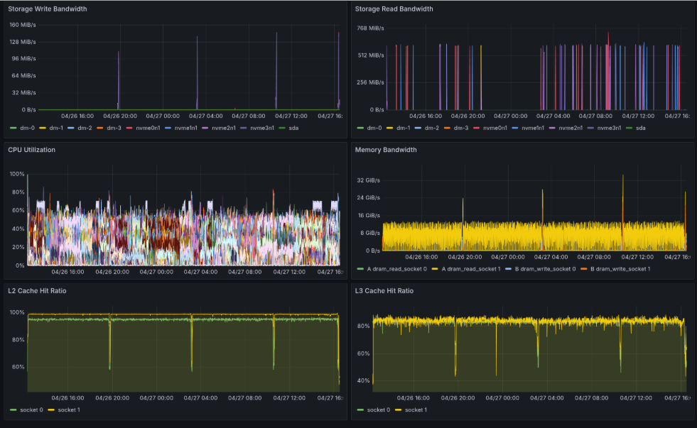
• Storage Write Bandwidth: Storage Write occurs synchronized with GPU stalls
• Storage Read Bandwidth: Storage Read occurs intermittently
• CPU Utilization: CPU has spare capacity

Flame Graph Analysis

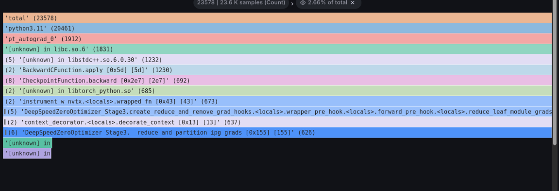
In the profile panel, clicking the Flame Graph button displays an enlarged flame graph. Focus on the pt_autograd_#N processing in the third row from the top. This PyTorch Engine thread occupies the majority of processing time. Also, focusing on the lower section of each pt_autograd_#N, the processing is divided into two parts. First, let's examine the processing on the left side. Left-click on the processing outlined in white in the figure below, and click Focus Block in the tab that appears to see the details.

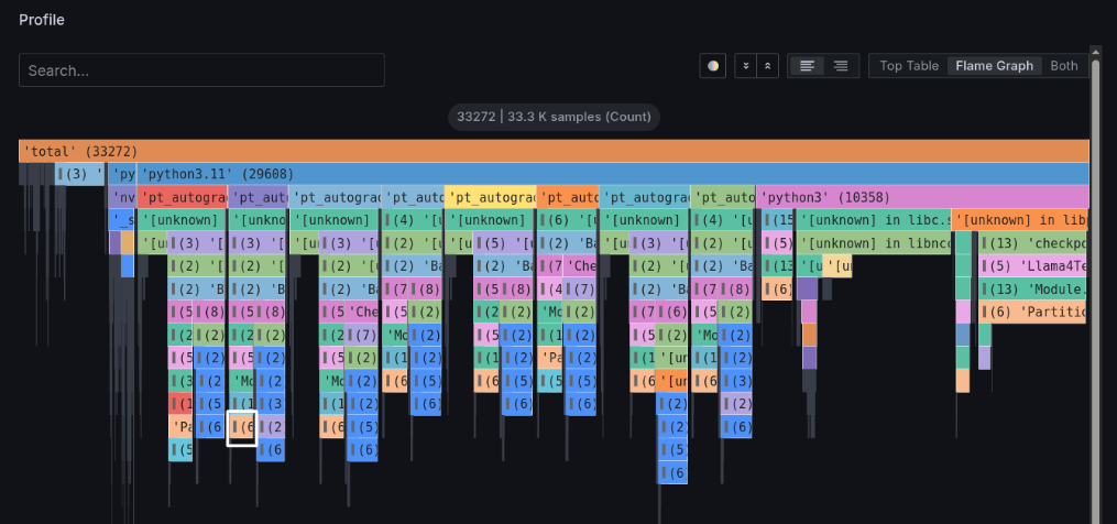
Looking at the figure below, it's blocked in the DeepSpeed fetch_sub_module function. From this code, we can predict that it's waiting for the arrival of parameters distributed across nodes.

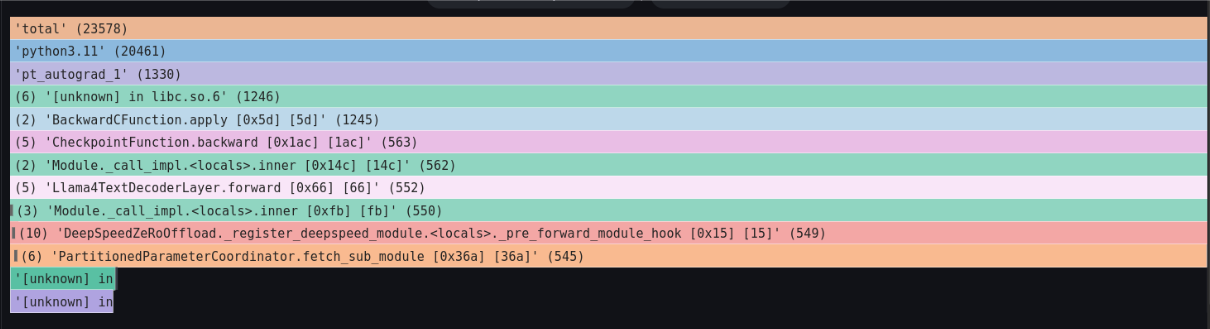
Next, let's examine the processing on the right side of the lower section of pt_autograd_#N. Left-click on the processing outlined in white in the figure below, and click Focus Block that appears to see the details.

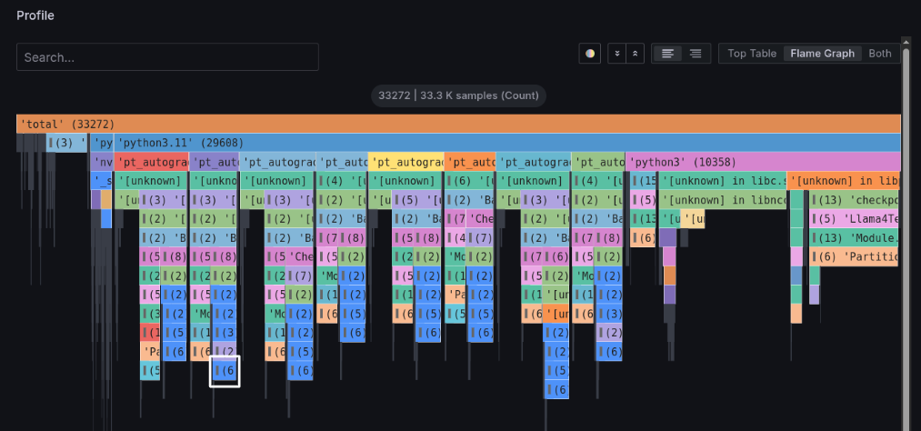
It's blocked in the DeepSpeed ZeRo3 _reduce_and_partition_ipg_grads function. From this code, we can predict that it's waiting for the completion of model gradient aggregation.

Analysis Summary

From the analysis of metrics and flame graphs above, we found the following:

• Unable to utilize full GPU power
• There are GPU stalls that appear to be checkpoint writing, but the overall impact is minimal
• Combining flame graph and code information, there's a possibility of blocking due to aggregation of data distributed across nodes
• However, interconnect bandwidth has spare capacity

From these observations, we can hypothesize that communication efficiency in distributed training is the bottleneck. Specifically, we infer that in DeepSpeed ZeRO3 parameter distribution and aggregation processing, communication wait time exceeds computation time.

Improvement Measure: Optimize DeepSpeed Hyperparameters

AIBooster includes tools for automatically tuning various DeepSpeed performance parameters.

We search for optimal values of DeepSpeed ZeRO3 configuration parameter sets to minimize execution time.

For detailed usage, please see the Performance Improvement Guide.

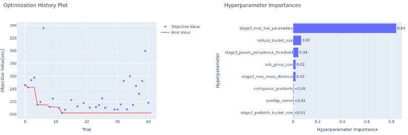
Optimization Results

Parameter Changes:

Parameter Name	Before Optimization	After Optimization
overlap_comm	false	false
contiguous_gradients	true	false
sub_group_size	1,000,000,000	14,714,186
reduce_bucket_size	26,214,400	1
stage3_prefetch_bucket_size	23,592,960	473,451
stage3_param_persistence_threshold	51,200	4,304,746
stage3_max_live_parameters	1,000,000,000	6,914,199,685
stage3_max_reuse_distance	1,000,000,000	3,283,215,516

Performance Improvement Results:

• Processing time: 50[s/itr] → 40[s/itr] (approx. 20% improvement)
• Communication bandwidth: 6.0 → 7.5[GiB/s] (approx. 25% improvement)
• Average GPU SM Activity: 21% → 28% (approx. 7% improvement)
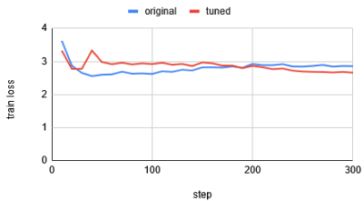
• No degradation observed in loss curve

With optimal parameters obtained through approximately 40 trials, training performance improved significantly.

Conclusion

By analyzing dashboard metrics and flame graphs, you can identify what to focus on for hyperparameter tuning (observation). Then, by using PI to search for optimal parameter set values, you can improve performance (improvement). In performance engineering, the loop of observation and improvement as described above is essential.

What is the bottleneck varies by environment and application. First, let's easily observe performance using the dashboard.

Reference Links

• DeepSpeed ZeRO: Memory Optimizations Toward Training Trillion Parameter Models